Estimating Regression Beta Using Excel Data Analysis Function

Note: Make sure that Data Analysis Add-on is installed with Excel. If not, follow the tutorial Video on YouTube.

Step 1: Getting historical data

Retrieve historical data of scrip price values and benchmark index value for a certain period of time. More the number of observations better it is, as it reduces standard error.

For this tutorial, Monthly closing price for share of Tata Power Ltd. On BSE and Closing value of SENSEX, the BSE Benchmark Index is considered from April 2001 to June 2011, comprising of 122 observations each.

Step 2: Calculate monthly returns on scrip and Index.

Monthly returns for both scrip as well as index are to be calculated.

Formula:

Monthly Return for Month = (Closing Price of the current month – Closing Price of previous month) / Closing Price of previous month

The raw data table in Excel should look like as below,

Scrip: Tata Power Ltd.
Month	Sensex Close	Closing Price of Scrip	Monthly Market Return (X)	Monthly Scrip Return (Y)
Apr-01	3519.16	121.4
May-01	3631.91	146.3	3.20%	20.51%
Jun-01	3456.78	130.05	-4.82%	-11.11%
Jul-01	3329.28	127.4	-3.69%	-2.04%
Aug-01	3244.95	116.85	-2.53%	-8.28%
Sep-01	2811.6	100.3	-13.35%	-14.16%
Oct-01	2989.35	104.95	6.32%	4.64%
Nov-01	3287.56	122.95	9.98%	17.15%
Dec-01	3262.33	119.55	-0.77%	-2.77%
Jan-02	3311.03	115.45	1.49%	-3.43%
Feb-02	3562.31	119.3	7.59%	3.33%
Mar-02	3469.35	113.5	-2.61%	-4.86%
Apr-02	3338.16	111.9	-3.78%	-1.41%
May-02	3125.73	114.65	-6.36%	2.46%
Jun-02	3244.7	130.2	3.81%	13.56%
Jul-02	2987.65	103.85	-7.92%	-20.24%
Aug-02	3181.23	102.2	6.48%	-1.59%
Sep-02	2991.36	95.65	-5.97%	-6.41%

Step 3: Run Regression

Method 1: Using Data Analysis Tool

Go to Data Tab, Click ‘Data analysis’

Select Function ‘Regression’

Select market Return as ‘Input Y Range’ and Scrip Return as ‘Input X Range’. To obtain Regression Results on different worksheet/workbook, select appropriate option in Output Options section.

For Tata Power and Sensex Regression, Monthly Scrip Return (Green) is ‘Range Y input’ and Monthly Market Return (Blue) is ‘Range X Input’ as shown below.

Click ‘Ok’ to receive results as shown below,

SUMMARY OUTPUT
Regression Statistics
Multiple R	0.76592712
R Square	0.586644353
Adjusted R Square	0.583199723
Standard Error	0.076757061
Observations	122
ANOVA
	df	SS	MS	F	Significance F
Regression	1	1.003388077	1.003388	170.3069	8.99945E-25
Residual	120	0.706997563	0.005892
Total	121	1.71038564
	Coefficients	Standard Error	t Stat	P-value	Lower 95%	Upper 95%	Lower 95.0%	Upper 95.0%
Intercept	0.006620394	0.00710666	0.931576	0.353426	-0.007450298	0.020691086	-0.007450298	0.020691086
X Variable 1	1.188147579	0.091044613	13.05017	9E-25	1.007885583	1.368409574	1.007885583	1.368409574

X Variable 1 is the ‘Beta’ for the scrip.

For Tata Power Beta works out to be 1.188, while R-square is 58.66%.

Method 2: Using Scatter Plot

One can create a regression Beta in Excel using the chart functions. Since Beta is the slope in a regression where market returns are on the X axis and scrip returns are on the Y axis.

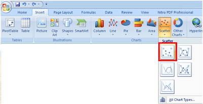
Select both Market return (as X) and scrip return (as Y) columns. Go to “Insert>Charts>Scatter”

The Chart should appear like this,

Select Chart, Go to ‘Layout tab’ and click ‘More Trendline options’.

Set the Checkboxes to show line equation and R-Square value on graph.

Final Output:

Slope of the line (1.1881) is ‘Beta’ of scrip.

Working Excel of the Tutorial can be downloaded from here.

Important Links

1.       YouTube - Excel Statistics 08: Install Excel 2007 Data Analysis Add-in http://www.youtube.com/watch?v=-ubtpQJ1smI

2.       Beta (Finance) (http://en.wikipedia.org/wiki/Beta_(finance))

3.       Linear Regression (http://en.wikipedia.org/wiki/Linear_regression)

Calculating Cost of Equity for an Indian Company

(Based on ‘Equity Risk Premiums (ERP): Determinants, Estimation and Implications – The 2011 Edition by Aswath Damodaran’.)

In capital Asset Pricing Model (CAPM) the expected return on asset/investment is calculated as,

Expected Return = Riskfree Rate + Beta_Asset (Equity Risk Premium)

So, to arrive at the expected return on an investment one needs to know following three parameters,

1. Riskfree Rate: The return on any risk free investments such as T-Bills, Sovereign Bonds etc. The time horizon for investment should match with the maturity of riskfree investment considered to get Riskfree Rate. So, if investor is planning for 6 months of time horizon Interest rate of a T-Bill will do; and if he/she is planning for longer duration, comparable GOI bond should be considered. It is important that for bonds ‘Bid Yield’ is considered as Riskfree rate and not coupon rate.

Note: Rate of T-Bills can be found at Reserve Bank of India’s site (http://www.rbi.org.in), in the section ‘Current rates>market Trends>Govt. Securities Market’.

Yield on bonds can be found at The Fixed Income Money Market and Derivatives Association of India’s website as Par yield on current date for the bond in consideration.

Mature markets like U.S., Germany which are AAA rated are considered with zero default risk in Govt. Securities, while markets like India, China, Brazil etc. Are considered riskier than mature markets and hence Govt. Securities issued by these countries are considered to carry default risk. (There have been incidents in the past when even Governments have defaulted on Bond payments, like default by Russian Govt. in 1990-91.)

Hence to arrive at Riskfree rates for markets like India, Country Risk Premium (CRP) is subtracted from Bond’s (Current yield) Rate.

CRP is dependent on Sovereign Rating of a country and volatility in Benchmark Bond & Benchmark Equity index yields.

Risk Free Rate = Yield on Benchmark Bond/T-Bill – Country Risk Premium

2. Beta_{Asset
To learn how to calculate Beta of an asset/scrip see,}
 Estimating Regression Beta Using Excel Data Analysis Function

3. Equity Risk Premium (ERP)

Risk premium to be charged for an investment not only reflects the nature of risk associated with the security but also risk arising out of investments in markets which themselves carry certain default risk. Thus, ERP for a market is calculated by adding ‘Default Spread’ for a country (which depends on Sovereign Rating of a country) to Premium on Equity investment in Mature Markets like U.S..

Equity Risk Premium = Mature Market Premium + Default Spread

Data about CRP, Default Spread, ERP, Sovereign Ratings etc. can be found on Prof. Aswath Damodaran’s Home Page (Damodaran Online).

Example

To calculate, Expected Return for ‘Tata Power Ltd.’

Date	19 June 2011
Country	India
Moody's Rating	Ba1
Default Spread	2.40%
Country Risk Premium for India	3.60%
For US (Mature Market) risk premium	5.00%
Equity Risk Premium for India	8.60%
(Mature market Premium + Default Spread)
Risk Free Rate
10 year GOI Sovereign Bond yield as on June 17, 2011	8.28%
Risk Free Rate (Bond Yield - Country Risk Premium)	4.68%
Cost of Equity
Firm	Tata Power Ltd.
Beta of Tata Power	1.1881
Cost of Equity for Tata Power Ltd.	14.90%
(CAPM: Cost of Equity = Riskfree Rate + BetaAsset (Equity Risk Premium)

Working Excel can be downloaded from here.

Links:

1. Damodaran Online (http://pages.stern.nyu.edu/~adamodar/)

2. ‘Equity Risk Premiums (ERP): Determinants, Estimation and Implications – The 2011 Edition by Aswath Damodaran’ (http://ssrn.com/abstract=1769064).

3. Important Excel functions for bond related calculations from RBI

(http://www.rbi.org.in/scripts/FAQView.aspx?Id=79#A4)

4. The Fixed Income Money Market and Derivatives Association of India

(http://www.fimmda.org)