What is R-Squared

As Investopedia states, it is a statistical measure that represents the percentage of a fund or security's movements that can be explained by movements in a benchmark index.

Thus it denotes the portion of a risk associated with a security that is market related.

Beta and R-Squared

While Beta measure how sensitive a security is to the Index movements, R-Squared denotes the co-relation between Index movements and Security price movements. Thus, Value of R-Squared equal to 1 denotes perfect correlation between Index and Security Price movements.

Beta in isolation is a useless number. It is essential to take a look at R-squared along with beta. The R-squared value shows how reliable the beta number is. Higher the R-Squared more reliable Beta is (Exceptions always possible).

Both Beta and R-Squared are directly affected by choice of index made. Hence it is always advisable to have a Broad based Index like S&P500 while calculating.

Jensen's alpha

Jensen's alpha is used to determine the return of a security or portfolio of securities over the theoretical expected return. Theoretical Return is calculated by models like CAPM etc.

In capital Asset Pricing Model (CAPM) the expected return on asset/investment is calculated as,

Expected Return = Riskfree Rate + Beta_Asset(Equity Risk Premium)

To calculate Jensen’s alpha one requires the following inputs:

realized return (on the security/portfolio),
market return,
risk-free rate of return, and
beta of the security/portfolio.

Jensen's alpha = Security or Portfolio Return − [Risk Free Rate + Security or Portfolio Beta * (Market Return − Risk Free Rate)]

Thus it can clearly be seen that CAPM takes into account the relative risk of an investment/security and calculate the Expected theoretical return while, Jensen’s Alpha calculates returns over and above theoretical returns. Thus, Positive Jensen’s Alpha means performance of Security above expectations while, negative Jensen’s Alpha means below expectations performance by the security.

Jensen’s Alpha is derived from purely historical numbers and hence essentially it should not affect the future investment decision. Still it is widely used to judge performance of Mutual Funds.

Example

*Statistics Summary*	*Tata Power*	*NTPC*	*Reliance Power*	*Adani Power*	*Power Grid Corp.*
R Square	0.5866	0.4809	0.6987	0.0213	0.4197
Beta	1.1881	0.7145	1.4971	0.1251	0.6694
CAPM Estimated Returns	14.90%	10.82%	17.56%	5.76%	10.44%
Actual Returns over the Period in consideration	917%	121%	-21%	3.99%	-32%
Period in Consideration for the Stock (Years)*	10.33	6.58	3.00	1.83	3.5833
Annulised Returns ((1 + Rate of Return)1/N) - 1	25%	13%	-7%	2%	-10%
Jensen's Alpha	10.27%	2.00%	-24.93%	-3.60%	-20.61%
*Refer Raw Data Sheet

Thus above example depicts the fact that investment in Tata Power has yielded more returns that theoretical estimations or say, expectations (of mine off course), historically.

Working Excel can be downloaded from here.

Links:

1. Investopedia R-Squared Definition (http://www.investopedia.com/terms/r/r-squared.asp#axzz1cacIVWMK)

2. Wikipedia Theory – Jensen’s Alpha (http://en.wikipedia.org/wiki/Jensen's_alpha)

Note: Make sure that Data Analysis Add-on is installed with Excel. If not, follow the tutorial Video on YouTube.

Step 1: Getting historical data

Retrieve historical data of scrip price values and benchmark index value for a certain period of time. More the number of observations better it is, as it reduces standard error.

For this tutorial, Monthly closing price for share of Tata Power Ltd. On BSE and Closing value of SENSEX, the BSE Benchmark Index is considered from April 2001 to June 2011, comprising of 122 observations each.

Step 2: Calculate monthly returns on scrip and Index.

Monthly returns for both scrip as well as index are to be calculated.

Formula:

Monthly Return for Month = (Closing Price of the current month – Closing Price of previous month) / Closing Price of previous month

The raw data table in Excel should look like as below,

Scrip: Tata Power Ltd.
Month	Sensex Close	Closing Price of Scrip	Monthly Market Return (X)	Monthly Scrip Return (Y)
Apr-01	3519.16	121.4
May-01	3631.91	146.3	3.20%	20.51%
Jun-01	3456.78	130.05	-4.82%	-11.11%
Jul-01	3329.28	127.4	-3.69%	-2.04%
Aug-01	3244.95	116.85	-2.53%	-8.28%
Sep-01	2811.6	100.3	-13.35%	-14.16%
Oct-01	2989.35	104.95	6.32%	4.64%
Nov-01	3287.56	122.95	9.98%	17.15%
Dec-01	3262.33	119.55	-0.77%	-2.77%
Jan-02	3311.03	115.45	1.49%	-3.43%
Feb-02	3562.31	119.3	7.59%	3.33%
Mar-02	3469.35	113.5	-2.61%	-4.86%
Apr-02	3338.16	111.9	-3.78%	-1.41%
May-02	3125.73	114.65	-6.36%	2.46%
Jun-02	3244.7	130.2	3.81%	13.56%
Jul-02	2987.65	103.85	-7.92%	-20.24%
Aug-02	3181.23	102.2	6.48%	-1.59%
Sep-02	2991.36	95.65	-5.97%	-6.41%

Step 3: Run Regression

Method 1: Using Data Analysis Tool

Go to Data Tab, Click ‘Data analysis’

Select Function ‘Regression’

Select market Return as ‘Input Y Range’ and Scrip Return as ‘Input X Range’. To obtain Regression Results on different worksheet/workbook, select appropriate option in Output Options section.

For Tata Power and Sensex Regression, Monthly Scrip Return (Green) is ‘Range Y input’ and Monthly Market Return (Blue) is ‘Range X Input’ as shown below.

Click ‘Ok’ to receive results as shown below,

SUMMARY OUTPUT

Regression Statistics
Multiple R	0.76592712
R Square	0.586644353
Adjusted R Square	0.583199723
Standard Error	0.076757061
Observations	122

ANOVA
	df	SS	MS	F	Significance F
Regression	1	1.003388077	1.003388	170.3069	8.99945E-25
Residual	120	0.706997563	0.005892
Total	121	1.71038564

	Coefficients	Standard Error	t Stat	P-value	Lower 95%	Upper 95%	Lower 95.0%	Upper 95.0%
Intercept	0.006620394	0.00710666	0.931576	0.353426	-0.007450298	0.020691086	-0.007450298	0.020691086
X Variable 1	1.188147579	0.091044613	13.05017	9E-25	1.007885583	1.368409574	1.007885583	1.368409574

X Variable 1 is the ‘Beta’ for the scrip.

For Tata Power Beta works out to be 1.188, while R-square is 58.66%.

Method 2: Using Scatter Plot

One can create a regression Beta in Excel using the chart functions. Since Beta is the slope in a regression where market returns are on the X axis and scrip returns are on the Y axis.

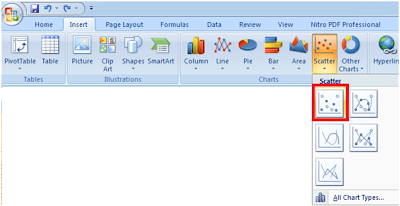
Select both Market return (as X) and scrip return (as Y) columns. Go to “Insert>Charts>Scatter”